
"It's all about bucks, kid. The rest is conversation."
Gordon Gekko
Wall Street (1987), directed by Oliver Stone

Money Never Sleeps
- 2 oz Standard Wormwood Rye whiskey
- ½ oz Punt E Mes
- ½ oz Cherry Heering
- 1 oz Sixpoint Brewery Resin Double IPA
- Garnish: Amarena cherry & grapefruit peel
Risk exposure: 3 units of alcohol
Recipes for Leverage
Mini-futures, constant leverage certificates, warrants and spread warrants — how to amplify returns, and the risks that come with it.
Wall Street is a Hollywood classic whose main character — the fictional broker Gordon Gekko — became a symbol of Wall Street greed. The sequel's title, Money Never Sleeps, gave its name to the cocktail above.
Yet there are important lessons in Gekko's approach: the difference between gambling and calculated risk-taking. Gekko doesn't gamble — he invests only after doing sufficient research to understand his odds. "I don't throw darts at a board. I bet on sure things. Read Sun Tzu, The Art of War. Every battle is won before it is ever fought." This is particularly important for leveraged products, which require a thorough understanding of risk and performance — especially the leverage and value-at-risk measures covered in Chapter 1.
Leverage means the product's value moves by more than 1% per percentage move in the underlying asset. It can be achieved in two ways: by borrowing capital (mini-futures, constant leverage certificates) or by using options (warrants, spread warrants). The SSPA Swiss Derivative Map classifies leverage products as the highest-risk of the four main structured product categories.
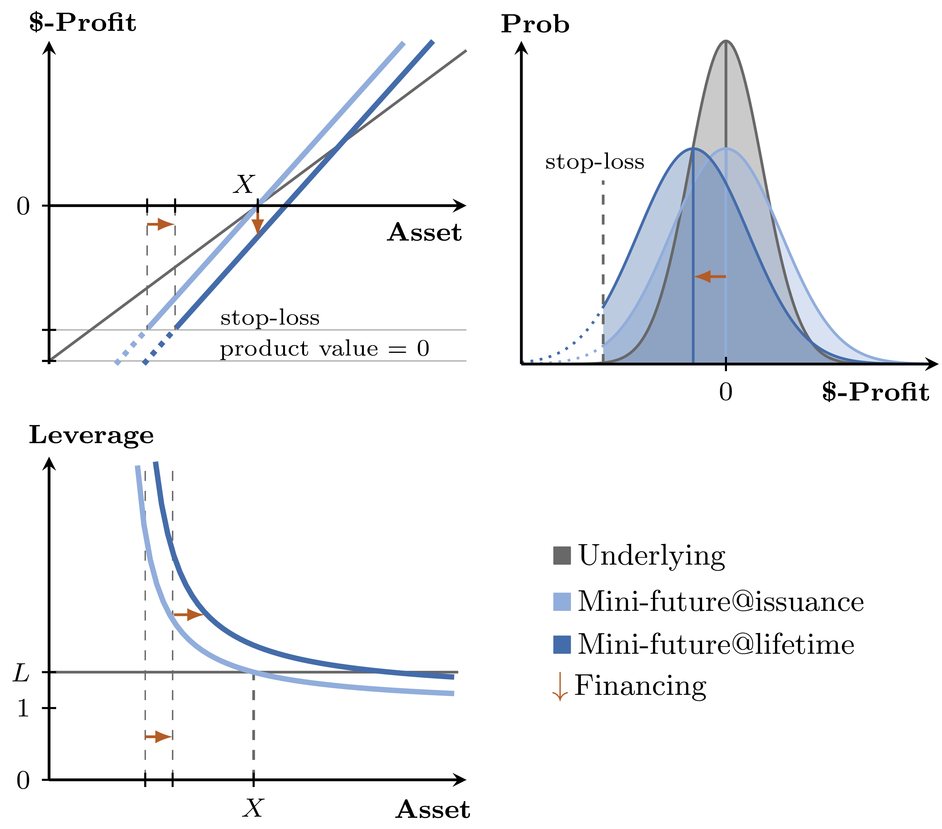
A mini-future achieves leverage by borrowing capital invested alongside the initial capital into the risky asset. A leverage of 2 means borrowing 100 for every 100 invested, buying 200 of the asset. If the asset rises 50%, the portfolio moves to 300 — a 100% gain on the initial capital (minus interest). If the asset falls 50%, the entire initial capital is wiped out.
The return formula for a mini-future with leverage L at time t is:
where $R_t$ is the accrued interest (financing cost) until time $t$. Since the product could in principle lose more than the investor's initial capital, issuers set a stop-loss limit that triggers product termination when the product value approaches zero. The stop-loss must be increased over time as interest accrues. The leverage itself is not constant — it changes as the asset price moves:
This means leverage increases when the product value falls — the product becomes riskier as it loses money.
Payoff at issuance and during investment period
Product parameters
| Strike X | At the money at issuance |
| Leverage (>1) | Leverage at issuance |
Replicating portfolio
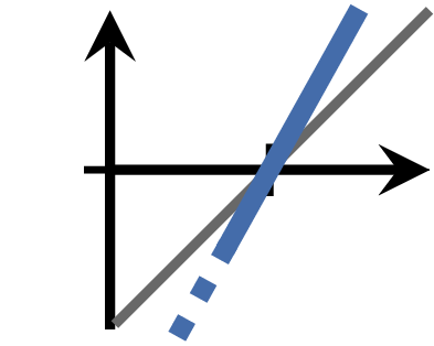
Borrow (L−1) × the initial capital in the money market to invest L × into the asset.
 Mini-Future
 Asset
Asset Money
MoneyMarket
Money market accrues interest (financing), reducing the product value and increasing the stop-loss asset price level over time.
Risk matrix
| Return | Long mini-future | Short mini-future |
|---|---|---|
| Profit | Asset↑ | Asset↓ |
| Loss | Asset↓ | Asset↑ |
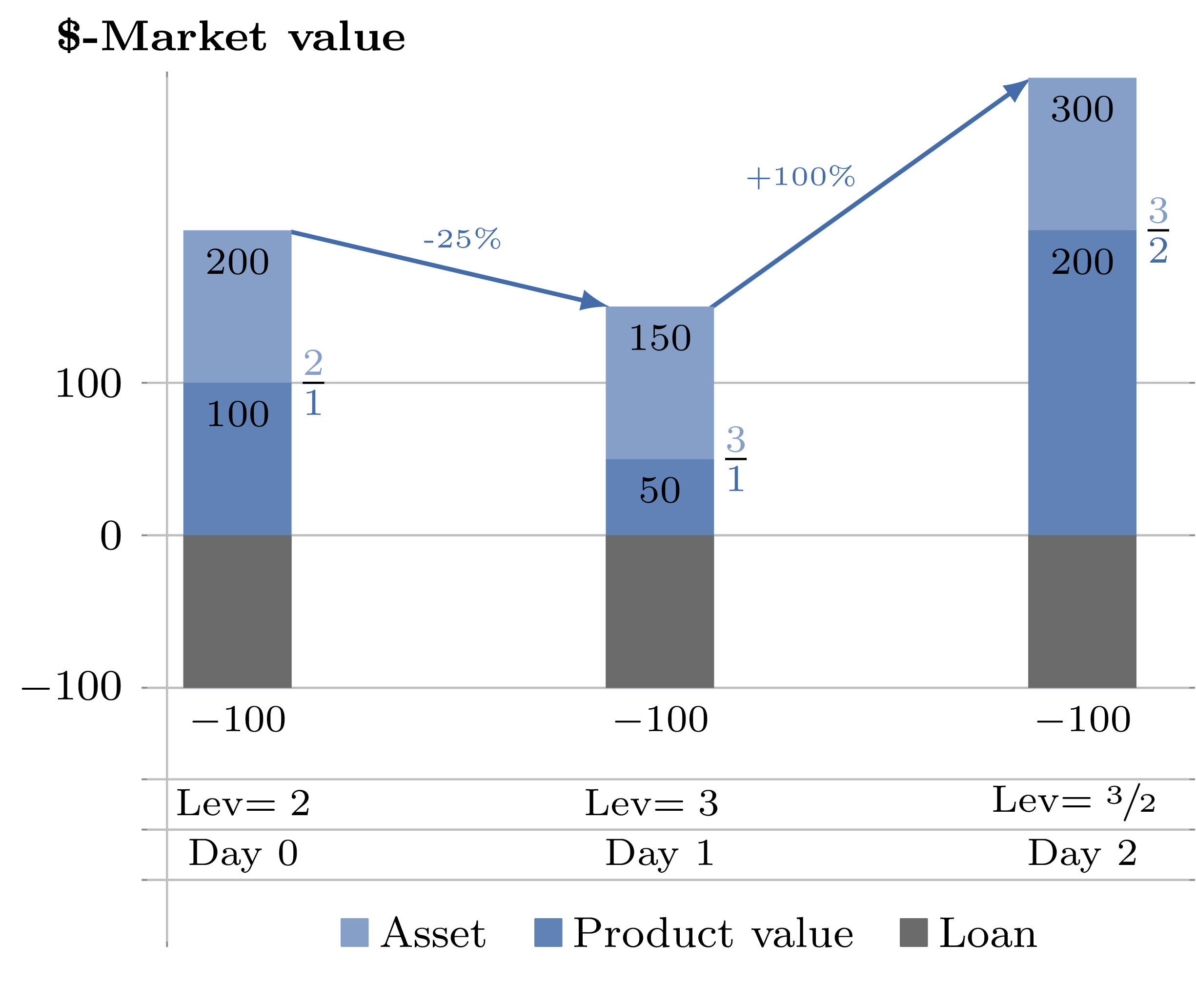
Daily performance of a mini-future with leverage 2. Arrows indicate asset returns. Ratios show the mini-future's leverage = total asset value ÷ product value. As the asset price moves, the leverage fluctuates — rising when the product value falls.
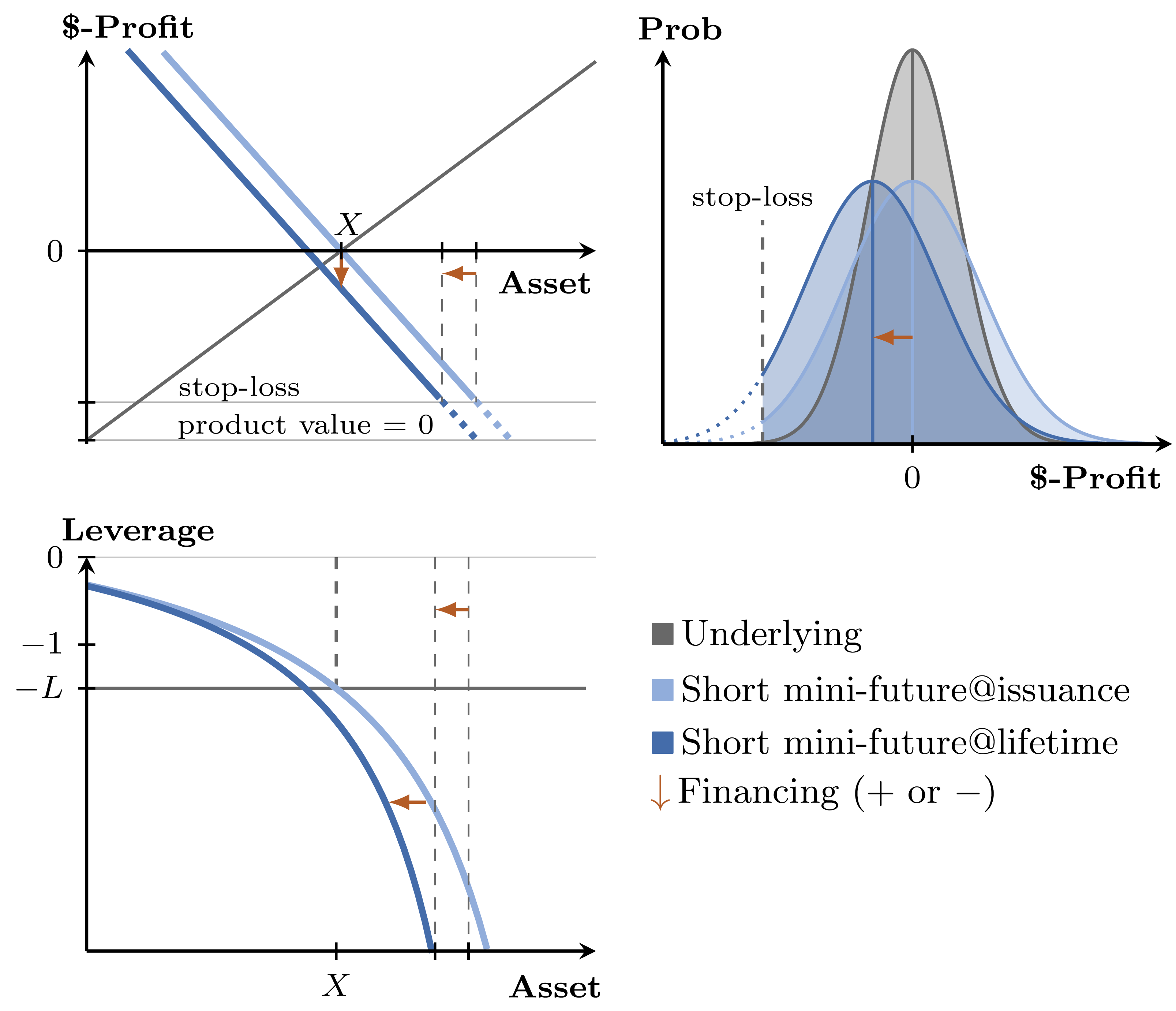
The short mini-future mirrors the long version — it short-sells the asset and invests the proceeds plus the initial capital into the money market. With short leverage L, it short-sells L × the asset and invests (L+1) × into the money market. Refinancing consists of borrowing fees (negative) and interest earned (positive). The stop-loss here is a maximum rise in the underlying price.
Payoff at issuance and during investment period
Product parameters
| Strike X | At the money at issuance |
| Short Leverage (≥1) | Short leverage at issuance |
Replicating portfolio
Borrow and short-sell L × the asset and invest (L+1) × the investment amount into the money market.
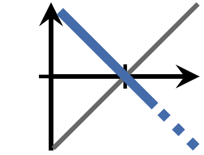 Short
ShortMini-Future
AssetMoneyMarket
Positive interest and negative borrowing fees accrue over time (financing, can be positive or negative), impacting the product value and stop-loss level.
The problem with mini-futures is that leverage fluctuates — and increases as the product loses value. Constant leverage certificates solve this by rebalancing the portfolio at the end of every trading day to keep the ratio of asset to loan constant at L:(L−1).
The rebalancing works as follows: after a day of negative returns, the issuer sells some of the asset to repay part of the loan — realising losses but restoring the ratio. After a positive day, the issuer borrows more and buys more asset. This creates an important side effect: if the asset zigzags sideways, the product continuously loses money through rebalancing losses. After three days of −20%, +50%, −16⅔% (cumulative asset return: 0%), the constant leverage certificate has lost 20%.
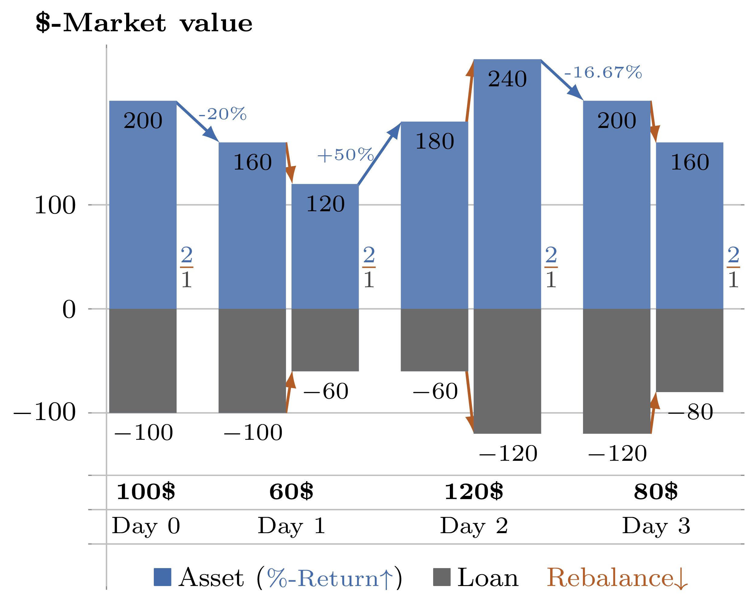
Daily asset moves and end-of-day rebalancing of a constant double leverage certificate. Dollar values show end-of-day product prices. After three days with zero cumulative asset return, the certificate has lost 20% due to rebalancing losses.
Payoff at issuance and during investment period
Product parameters
| Strike X | At the money at issuance |
| Leverage (>1) | Leverage at issuance — kept constant by daily rebalancing |
Replicating portfolio
Borrow (L−1) × the investment amount to invest L × into the asset. Rebalance daily to maintain ratio L:(L−1).
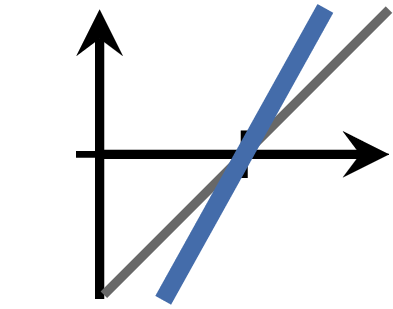 Constant
Leverage
AssetMoneyMarket
Financing costs and daily rebalancing losses accrue over time.
Risk matrix
| Return | One day | Long term |
|---|---|---|
| Outperformance | Asset↑ (linear) | Asset↑ (convex) |
| Underperformance & financing | Asset↓ (linear) | Rates↑, Vol↑ |
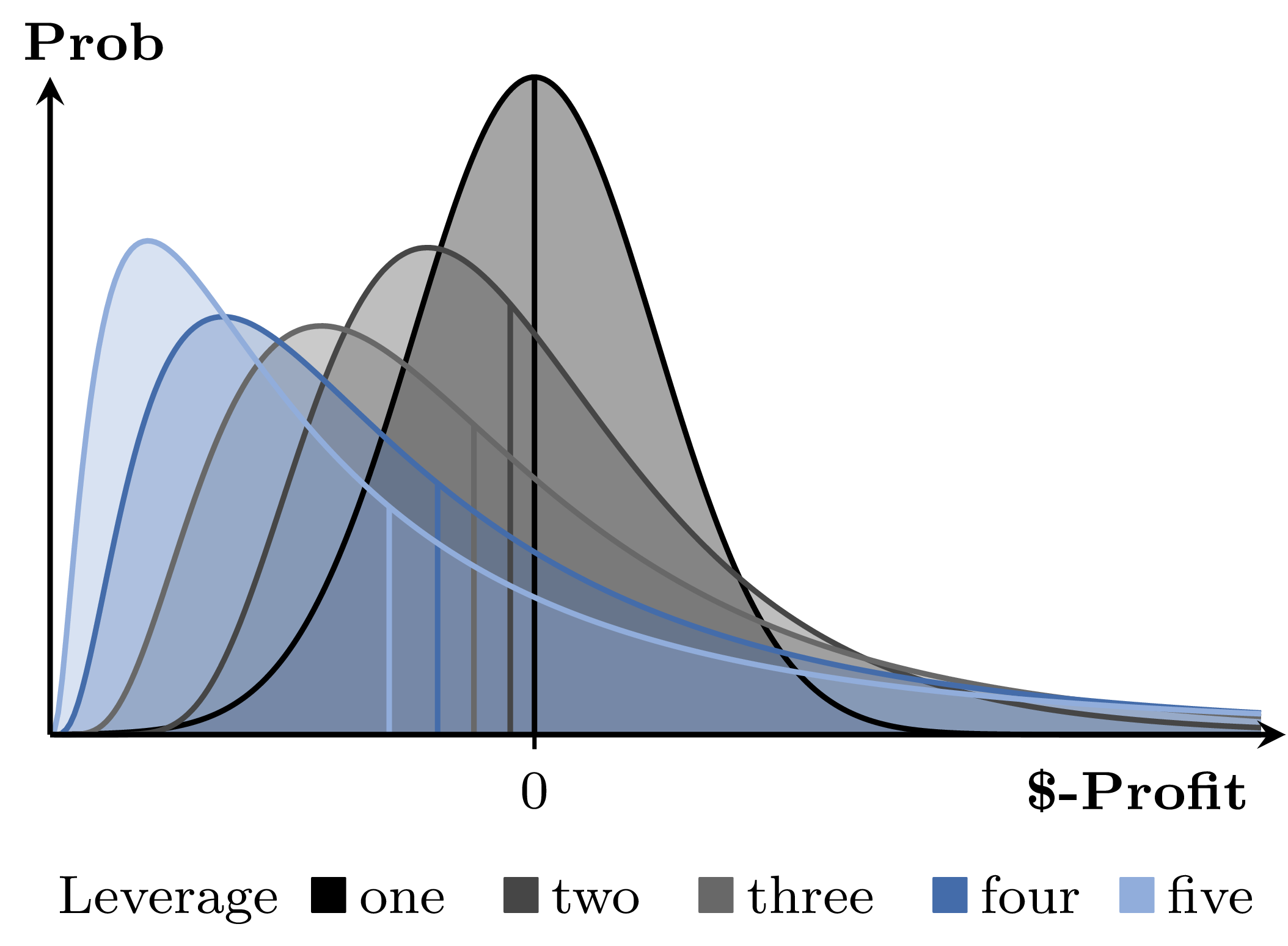
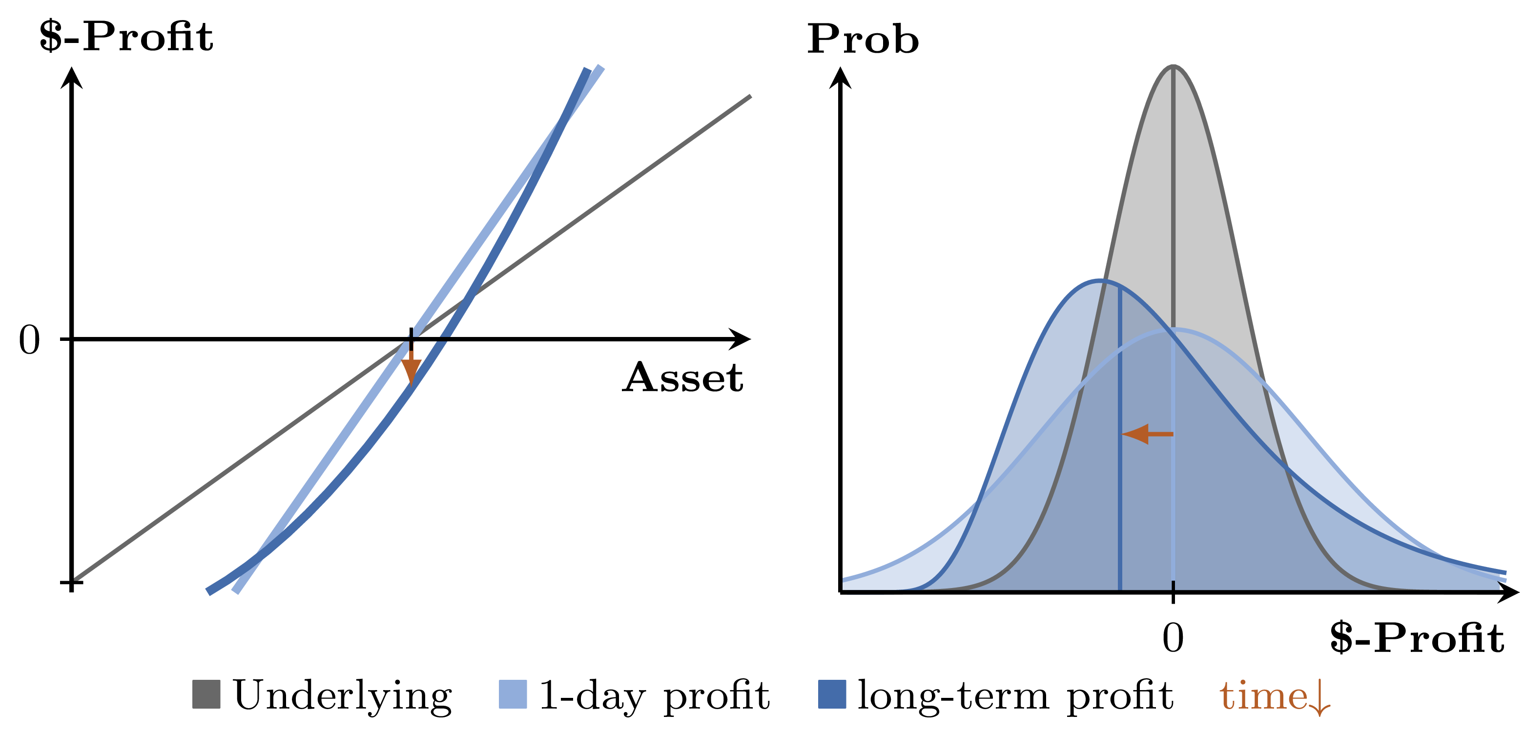
Probability distribution of different constant leverage certificates (vertical lines = median). Higher leverage produces a more right-skewed distribution reflecting greater convexity from daily rebalancing.
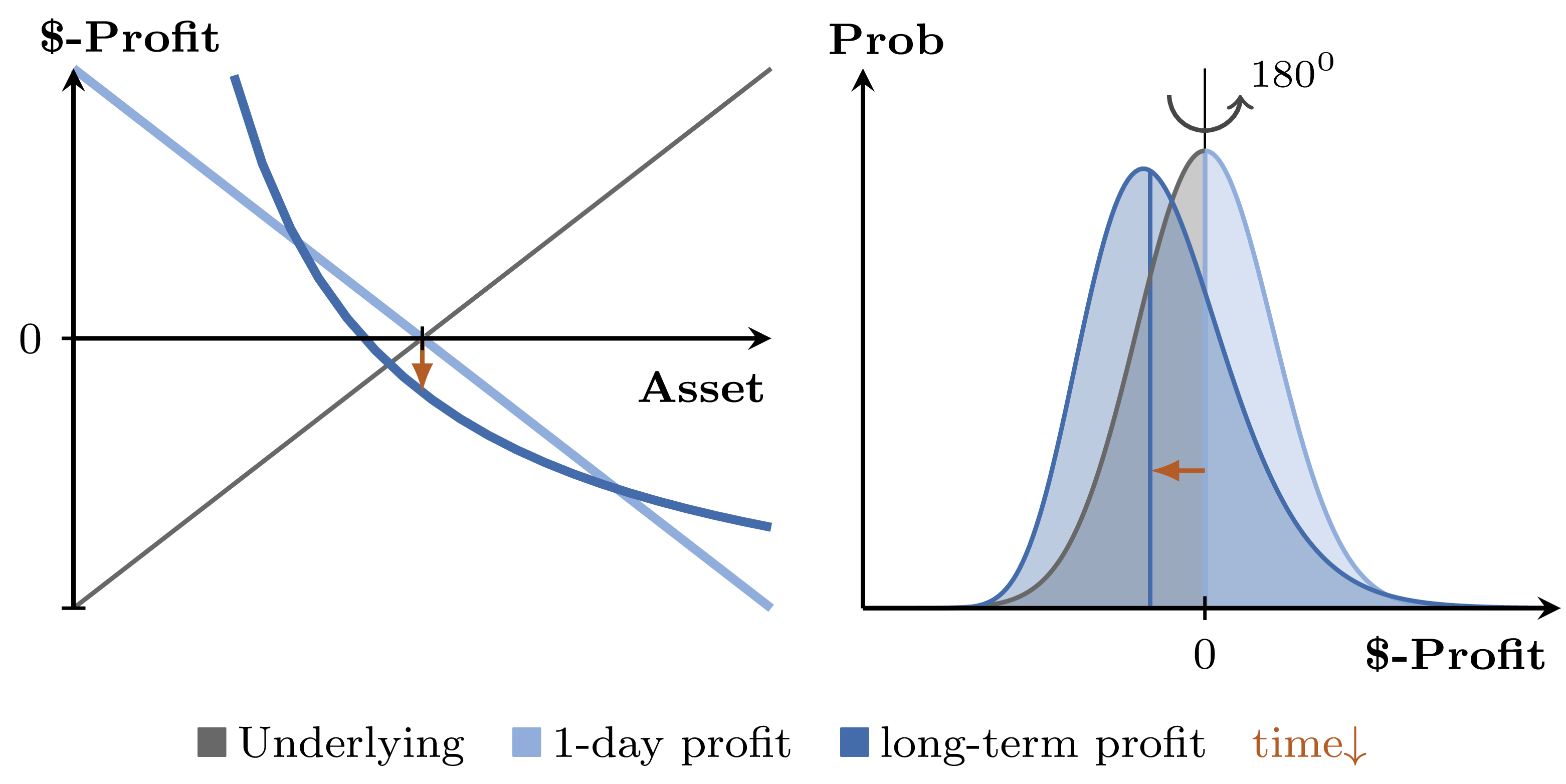
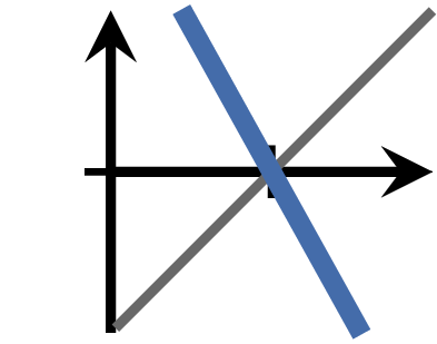
The short constant leverage certificate applies the same daily rebalancing logic to a short position — maintaining the ratio of short asset to money market at L:(L+1). The same compounding effect applies: the long-term payoff is convex, and zigzag markets create continuous rebalancing losses.
Payoff at issuance and during investment period
Product parameters
| Strike X | At the money at issuance |
| Short Leverage (≥1) | Short daily leverage — kept constant by daily rebalancing |
Replicating portfolio
Borrow and short-sell L × the asset and invest (L+1) × in the money market. Rebalance daily to ratio −L:(L+1).
 Constant
Short
AssetMoneyMarket
Financing costs and daily rebalancing losses accrue over time.
Risk matrix
| Return | One day | Long term |
|---|---|---|
| Outperformance | Asset↓ (linear) | Asset↓ (convex) |
| Underperformance & financing | Asset↑ (linear) | Rates↓, Vol↑ |
Mini-future vs Constant Leverage Certificate — the key distinction:
A mini-future has constant participation L and variable leverage over time.
A constant leverage certificate has constant leverage L and variable participation — maintained through daily rebalancing, which introduces path-dependency and rebalancing losses.
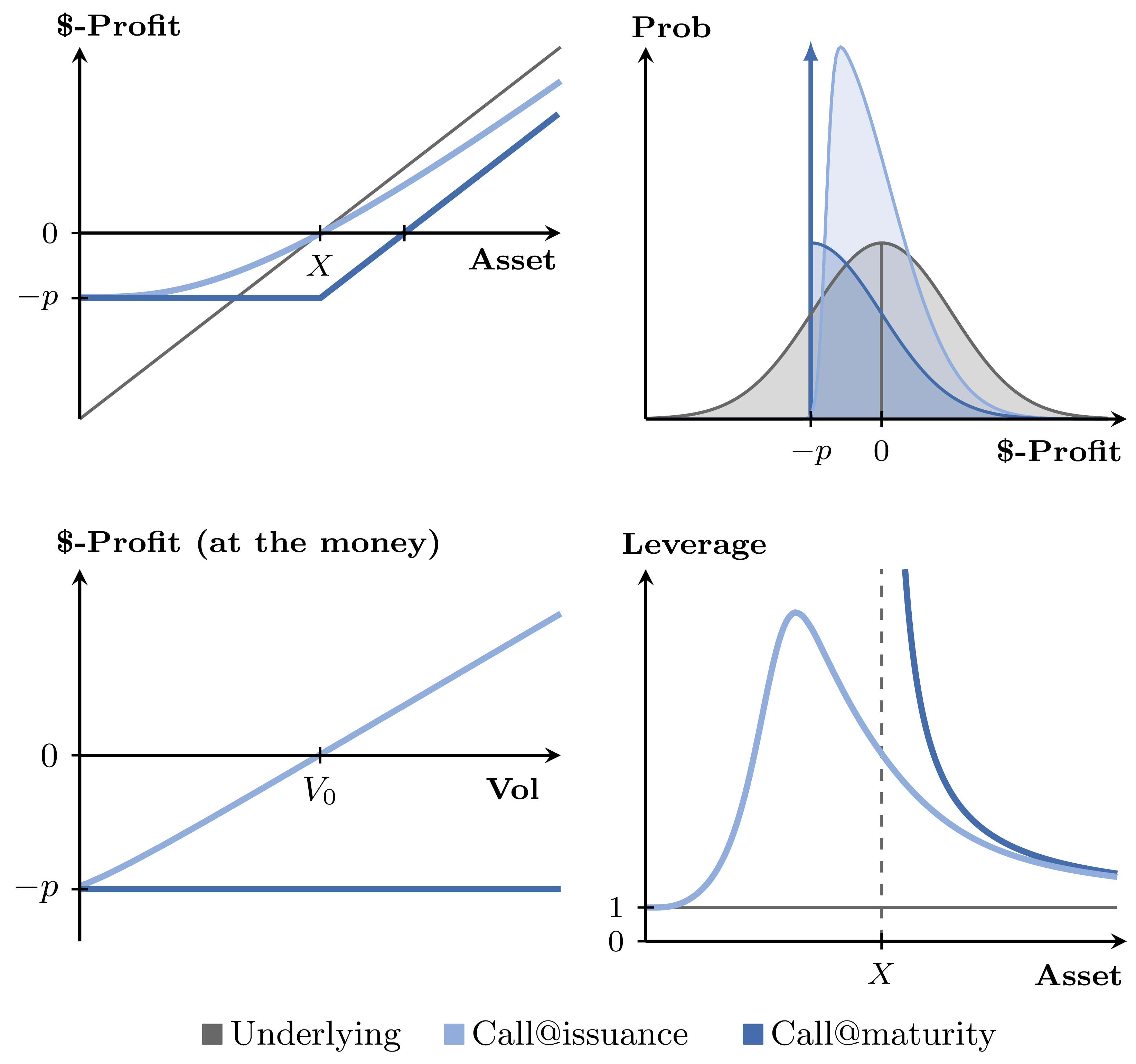
Call and put warrants are the "vodka and tequila shots" of financial markets — the most commonly used leveraged investment products. They are simply standard call and put options issued by a product provider. Both can lead to a 100% loss of the invested premium if they expire worthless. Warrant exchanges such as EUSIPA member exchanges publish standardised product information for investors.
Payoff at issuance and during investment period
Product parameters
| Strike X | Defined at issuance |
Replicating portfolio
The call warrant is identical to a standard call option.
Risk matrix
| Return | During lifetime | At maturity |
|---|---|---|
| Outperformance | Rates↑, Vol↑ | Asset > Strike |
| Forgone premium | Asset ≤ Strike | |
| Loss | Rates↓, Vol↓ | Asset ≤ Strike |
Payoff at issuance and during investment period
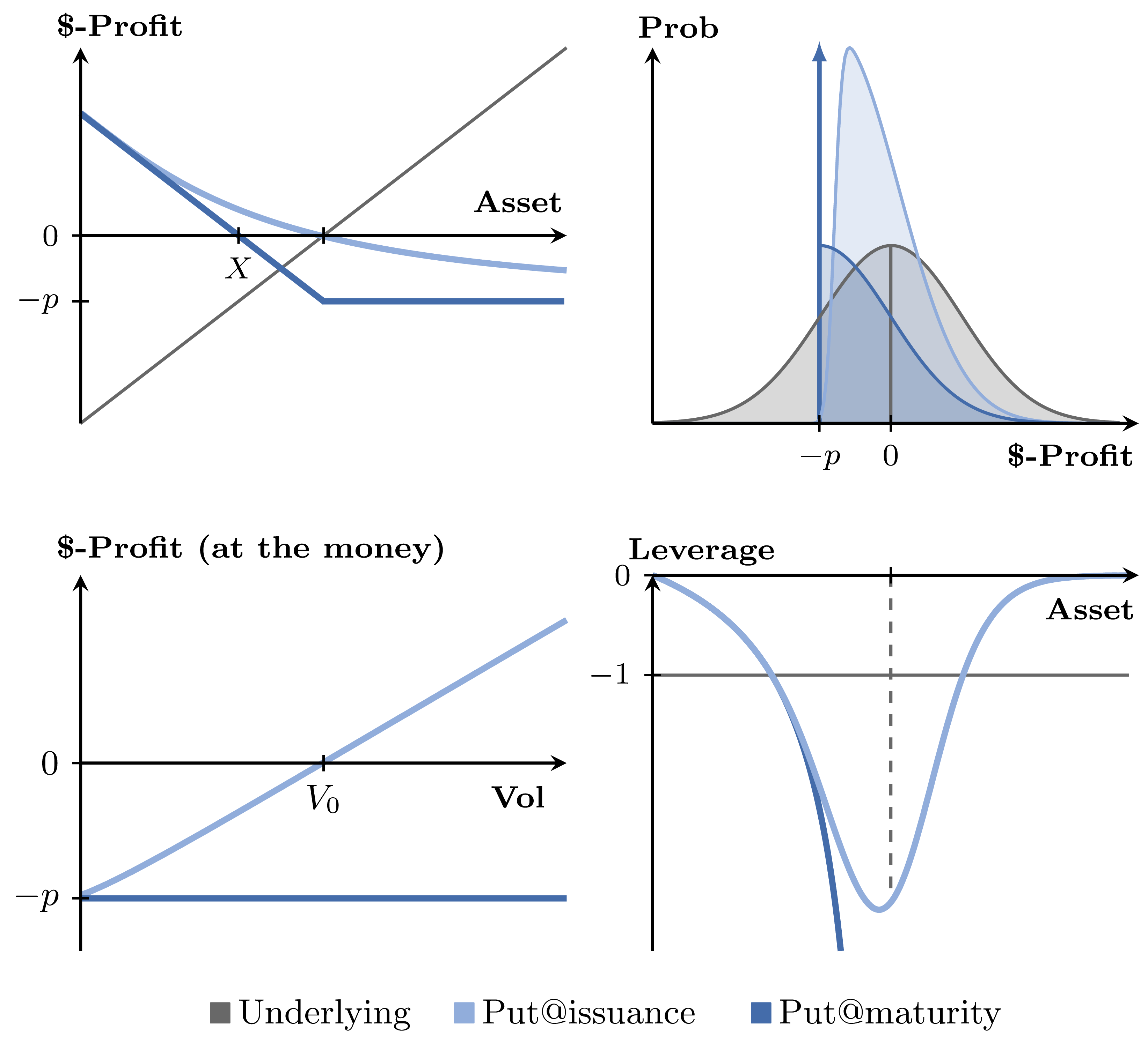
Product parameters
| Strike X | Defined at issuance |
Replicating portfolio
The put warrant is identical to a standard put option. Key difference from call: negative interest rate sensitivity (negative financing time value).
Risk matrix
| Return | During lifetime | At maturity |
|---|---|---|
| Outperformance | Rates↓, Vol↑ | Asset < Strike |
| Forgone premium | Asset ≥ Strike | |
| Loss | Rates↑, Vol↓ | Asset ≥ Strike |
Spread warrants are the "softened version" of call and put warrants — less alcohol, less expensive. They cap the upside at some point, making the option cheaper. Lower premium means lower losses if the option expires worthless.
Payoff at issuance and during investment period
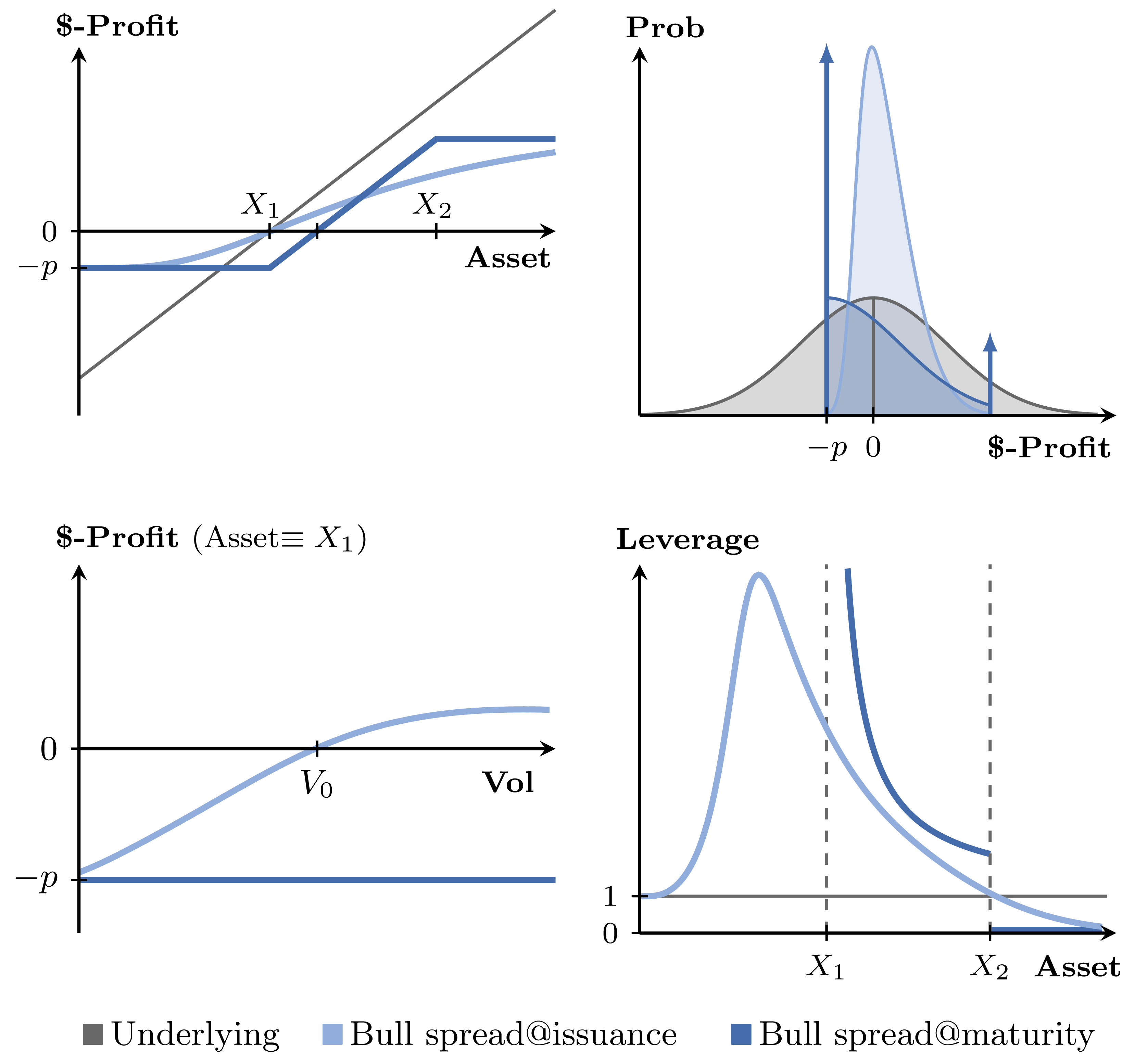
Product parameters
| Strike X₁ | Defined at issuance |
| Strike X₂ > X₁ | Defines the upside cap |
Replicating portfolio
Buy a call with strike X₁ and sell a call with strike X₂.
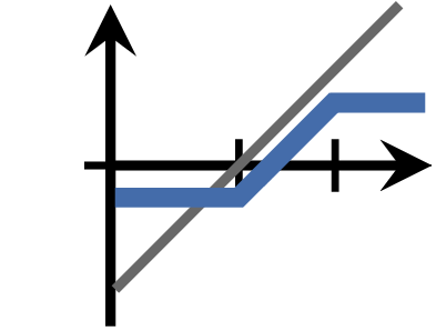 Bull Spread
 Call @ X₁
 Short Call
@ X₂
Risk matrix
| Return | During lifetime | At maturity |
|---|---|---|
| Outperformance | Rates↑, Vol↑ | X₁ < Asset ≤ X₂ |
| Forgone premium | Asset ≤ X₁ | |
| Loss | Rates↓, Vol↓ | Asset ≤ X₁ |
Payoff at issuance and during investment period
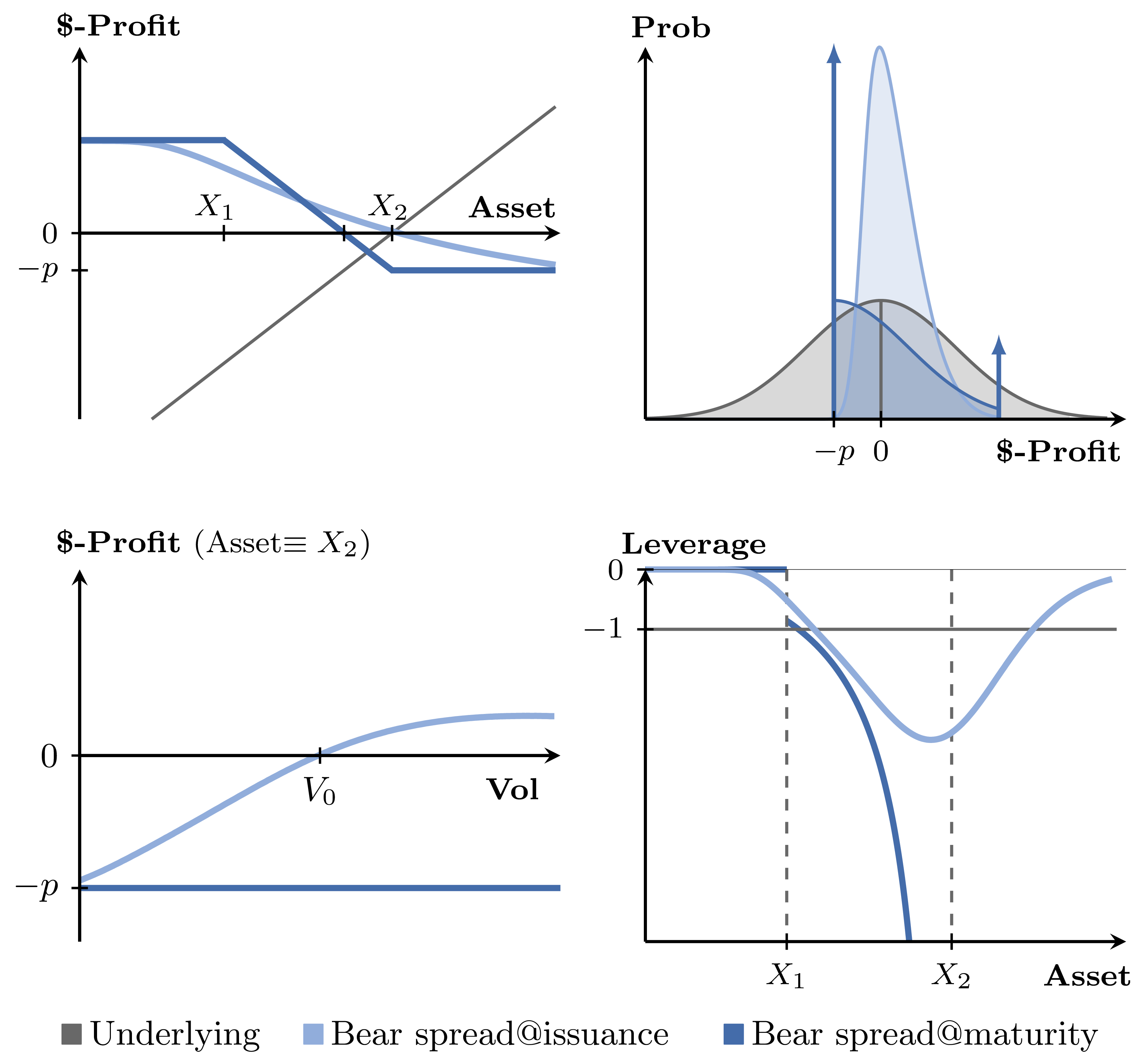
Product parameters
| Strike X₁ | Defined at issuance |
| Strike X₂ > X₁ | Defines the upside entry |
Replicating portfolio
Buy a put with strike X₂ and sell a put with strike X₁.
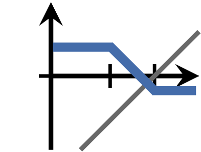 Bear Spread
 Short Put
@ X₁
 Put @ X₂
Risk matrix
| Return | During lifetime | At maturity |
|---|---|---|
| Outperformance | Rates↓, Vol↑ | Asset ≤ X₂ |
| Forgone premium | Asset ≥ X₂ | |
| Loss | Rates↑, Vol↓ | Asset ≥ X₂ |
A nice illustration of how modular structured products are — the capped capital-protected certificate (Chapter 4) can be replicated using a bull spread:
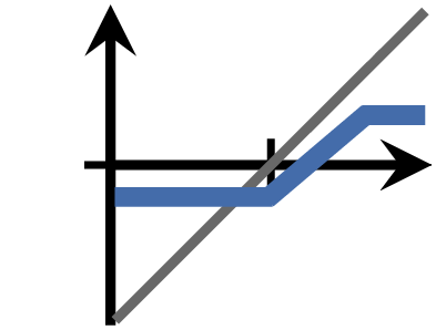 Capped Capital
Protected
Bull SpreadThe zero-bond's face value equals the bull spread's lower strike X₁. Like playing with Legos — complex products built from simpler ones.
- Leverage amplifies both profits and losses — as a rule of thumb, volatility and returns are multiplied by the leverage factor
- Mini-futures — constant participation, variable leverage; leverage increases as the product loses value; stop-loss terminates the product before total loss
- Constant leverage certificates — constant leverage, variable participation; daily rebalancing maintains the ratio but creates path-dependency and continuous rebalancing losses in sideways markets; not suitable for long-term investing (>1 year)
- Warrants — standard call or put options; can lead to 100% loss if they expire worthless; highest upside but also highest risk
- Spread warrants — capped versions of warrants; cheaper premium, capped upside; two probability spikes at maturity
- For strong directional bets with total-loss tolerance: warrants. For leveraged/short positions with residual value protection: constant leverage certificates — but avoid for long-term holding
Technical Appendix — The Compounding Effect of Constant Leverage
The key distinction in constant leverage certificates is between their one-day return (identical to a mini-future) and their long-term return (path-dependent, affected by rebalancing).
Daily return — for a constant leverage certificate with leverage L, the daily return is simply L times the daily asset return minus one-day financing costs:
Long-term return — over many trading days (typically >100), the performance can be approximated using just two parameters: the cumulative asset return and the average volatility over period T:
The exponential return arises because daily rebalancing amplifies upward trends (buying more when prices rise) and reduces downside exposure (selling when prices fall). The rebalancing loss is the cost of this process in sideways markets — it increases with volatility and with L.
For short constant leverage certificates with short leverage L ≥ 1:
The combination of the exponential return profile and the continuous rebalancing losses creates the compounding effect — the key performance difference between mini-futures and constant leverage certificates over time.
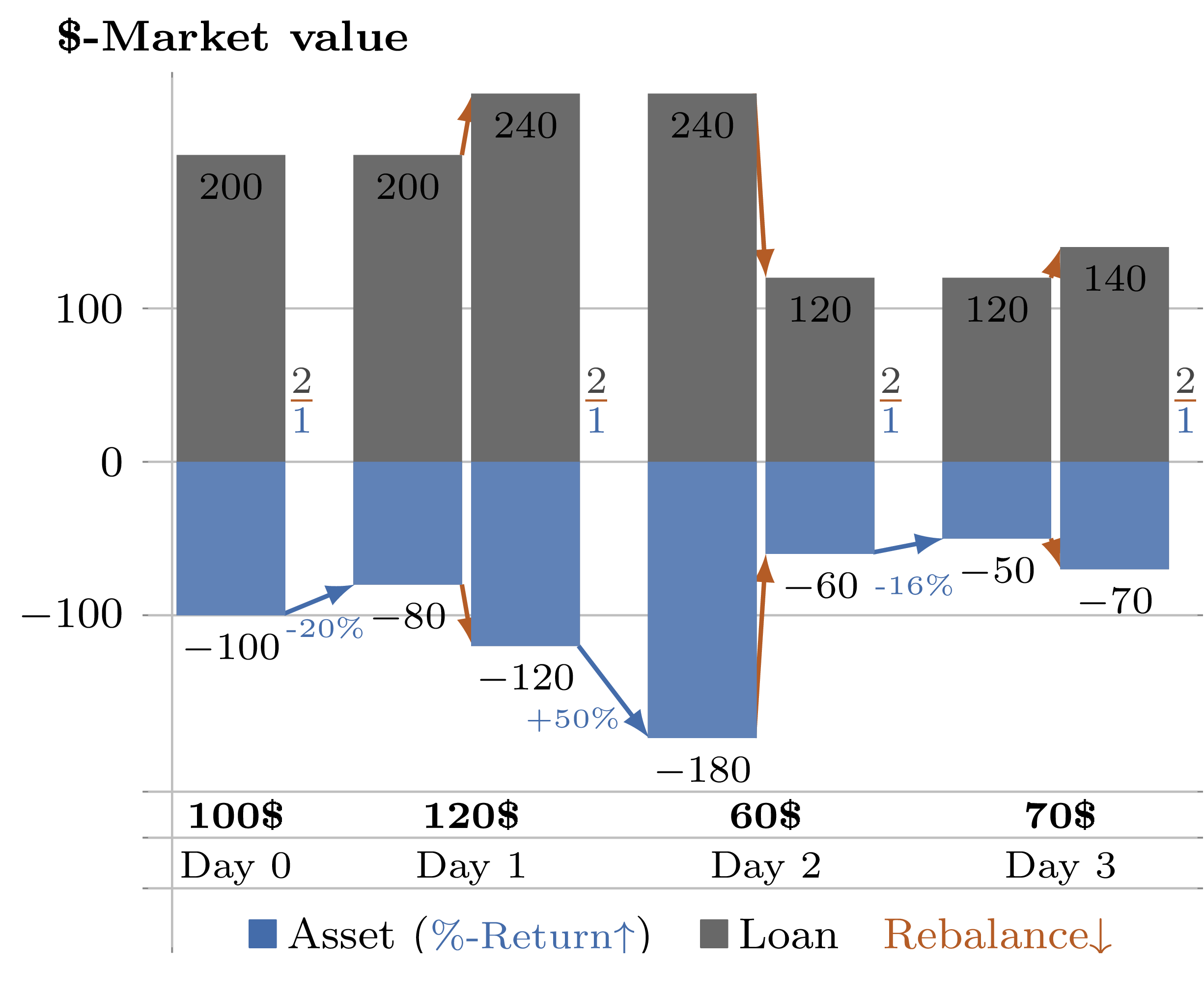
Daily asset price moves and end-of-day rebalancing for a constant short certificate. After three days with zero cumulative asset return, the constant short certificate has also lost value — the same compounding effect as the long constant leverage certificate.
Given the increased downside risk, it is essential to carefully scrutinise leveraged products and understand the size of potential losses before investing. Even with the best analysis, you may face a loss. For such a moment, two things to remember.
First, there is a cocktail for such moments:

The Stock Market Crash Cocktail
- ½ shot Jack Daniels
- ½ shot Yukon Jack
- ½ shot Southern Comfort
- ½ shot Wild Turkey
- ½ shot black rum
- Coca-Cola & ice cubes
Risk exposure: 4 units of alcohol — pour the Coke last, it does the stirring
Second, remember Gordon Gekko's advice:
"Don't run when you lose, don't whine when it hurts. It's like the first grade. No one likes a crybaby."
Gordon Gekko
Wall Street: Money Never Sleeps (2010)
For educational purposes only. Not investment advice. Derivative products carry significant risks and may not be suitable for all investors.