Index Derivative Strategies

Chapters 4–7 — product selection, payoff and risk charts, product settings and the structuring pane with rule modeller.

The Index Derivative Strategies pane allows you to create one or several structured products based on indexes and backtest them over time, including a regular roll-over of the product strategy to make the long-run performance analysis as realistic as possible. The four main product categories are explained in depth in the Derivative Academy.

The menu window below allows you to click through a selection of standard structured products in the tree selection on the left-hand side. Each new product you want to create starts by selecting a prototype from this list, which you can then modify.

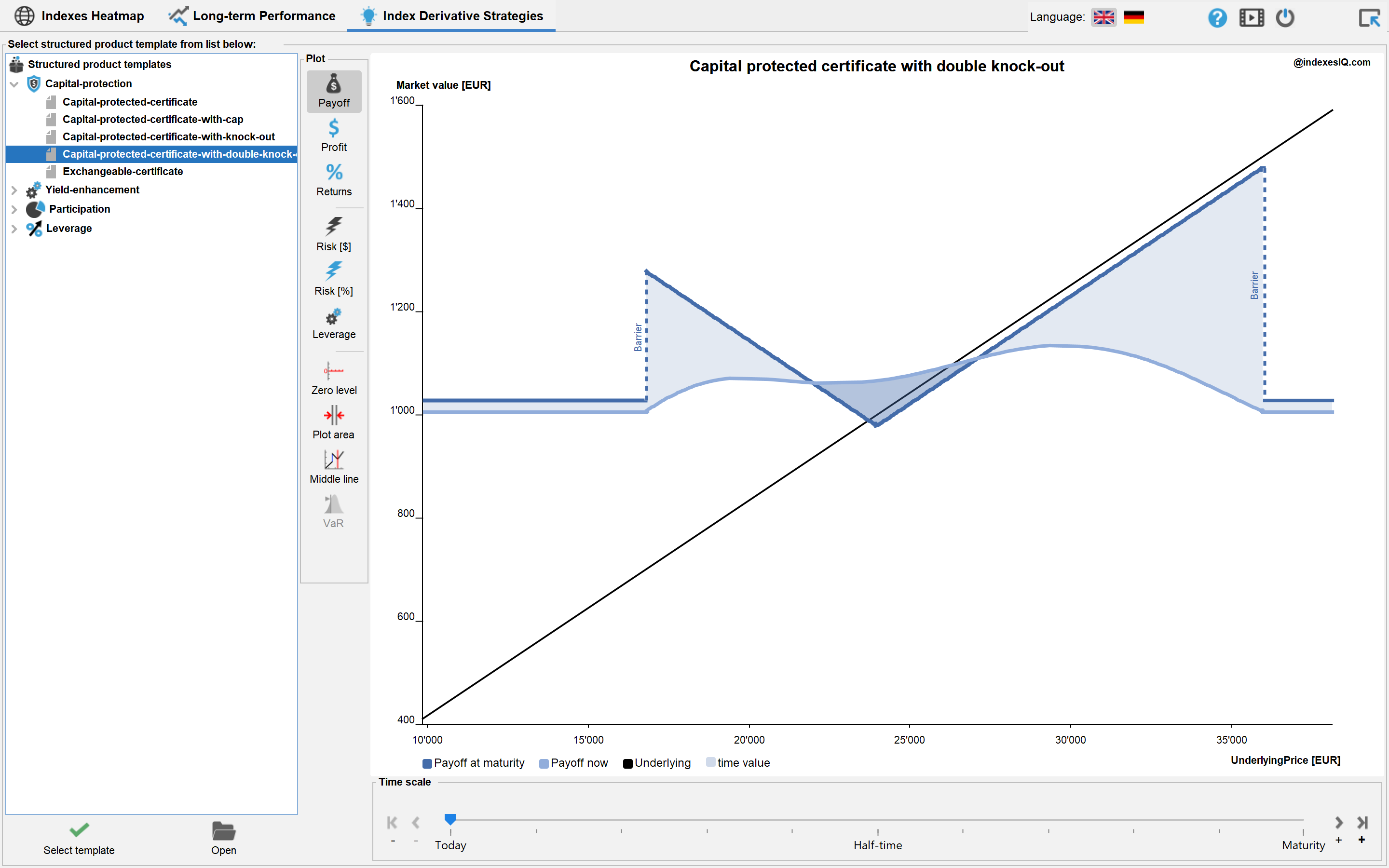
The selection of products is grouped into the four main product categories, shown in increasing order of investment risk — consistent with the SSPA Swiss Derivative Map classification:

These four categories are explained in detail in the Derivative Academy.

At the bottom of the window, the following functions are available:

Once you have selected a product, the window changes and the Select template button is replaced with new buttons:

Two additional functions are available in the menu below the chart:

• Product: Shows the menu of existing structured products in your portfolio and allows you to switch between them.
• The time scale function allows you to choose a time point between the issuance date and the maturity date of the product. The payoff plot or risk plot automatically adjusts to the chosen point in time.

Payoff Charts

Next to the payoff chart, you see a selection of plotting functions for the selected product:

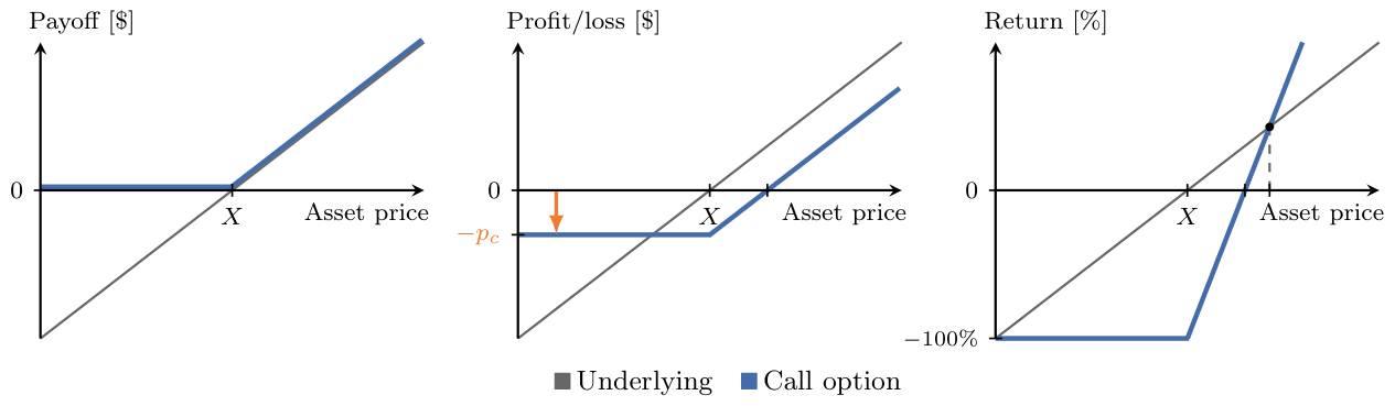
To understand these three plots conceptually, consider a standard call option purchased at option premium p_c. At maturity:

For a deeper conceptual explanation of these three measures, see Chapter 1 of the Derivative Academy.

Risk Charts

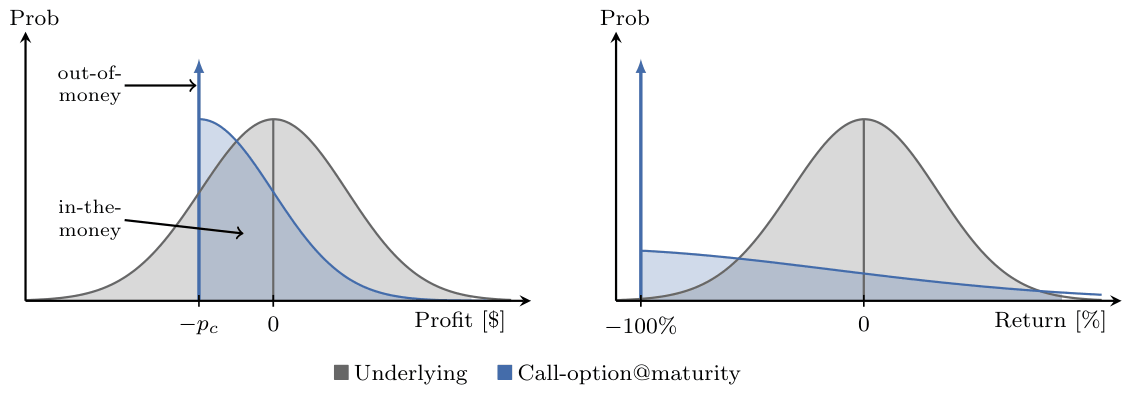
In addition to the performance-related plots, three risk-related plotting functions are available:

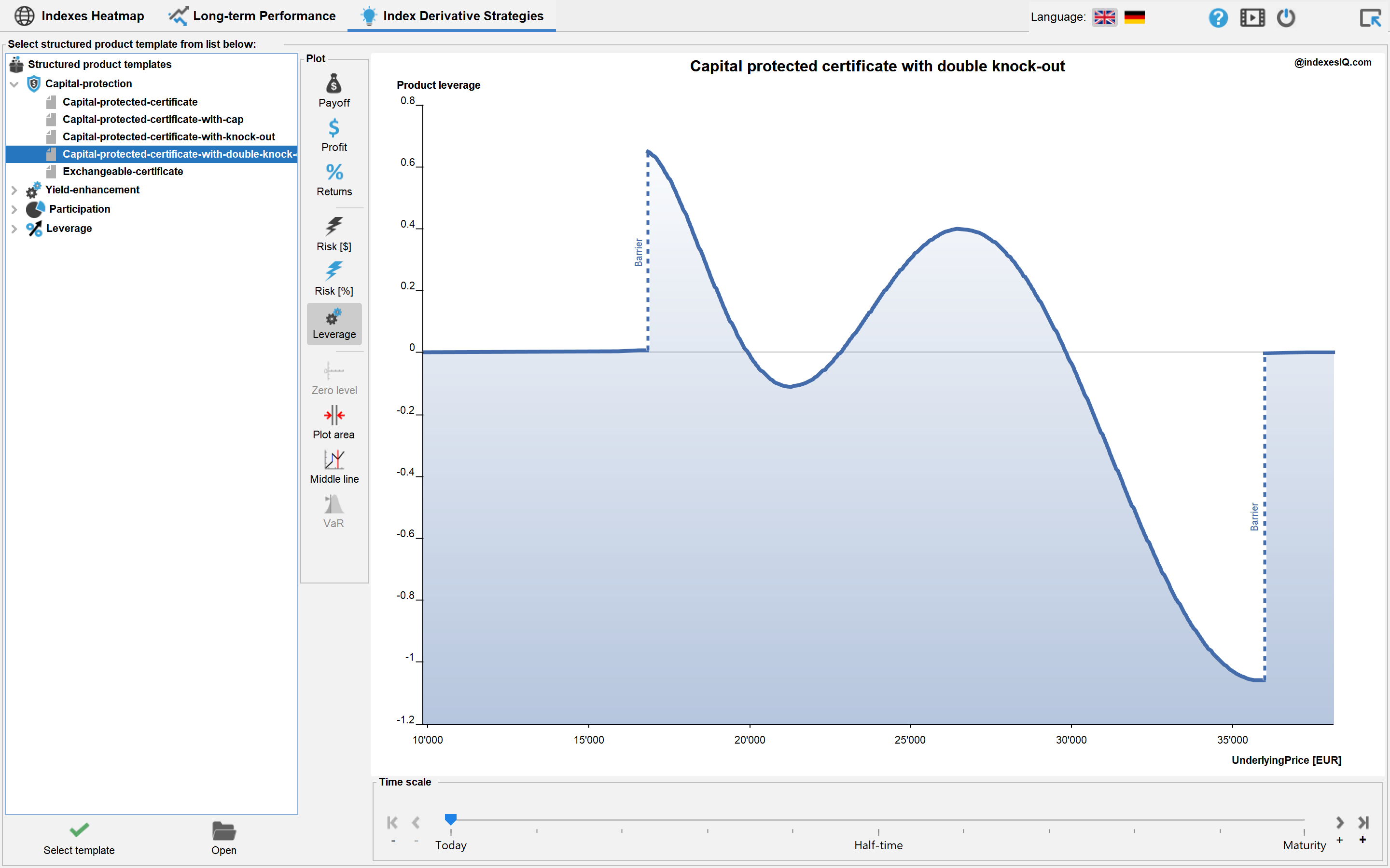
The leverage ratio is defined as the product's percentage change in value per percentage change in the value of the underlying:

Additional plot options for fine-tuning payoff and risk charts:

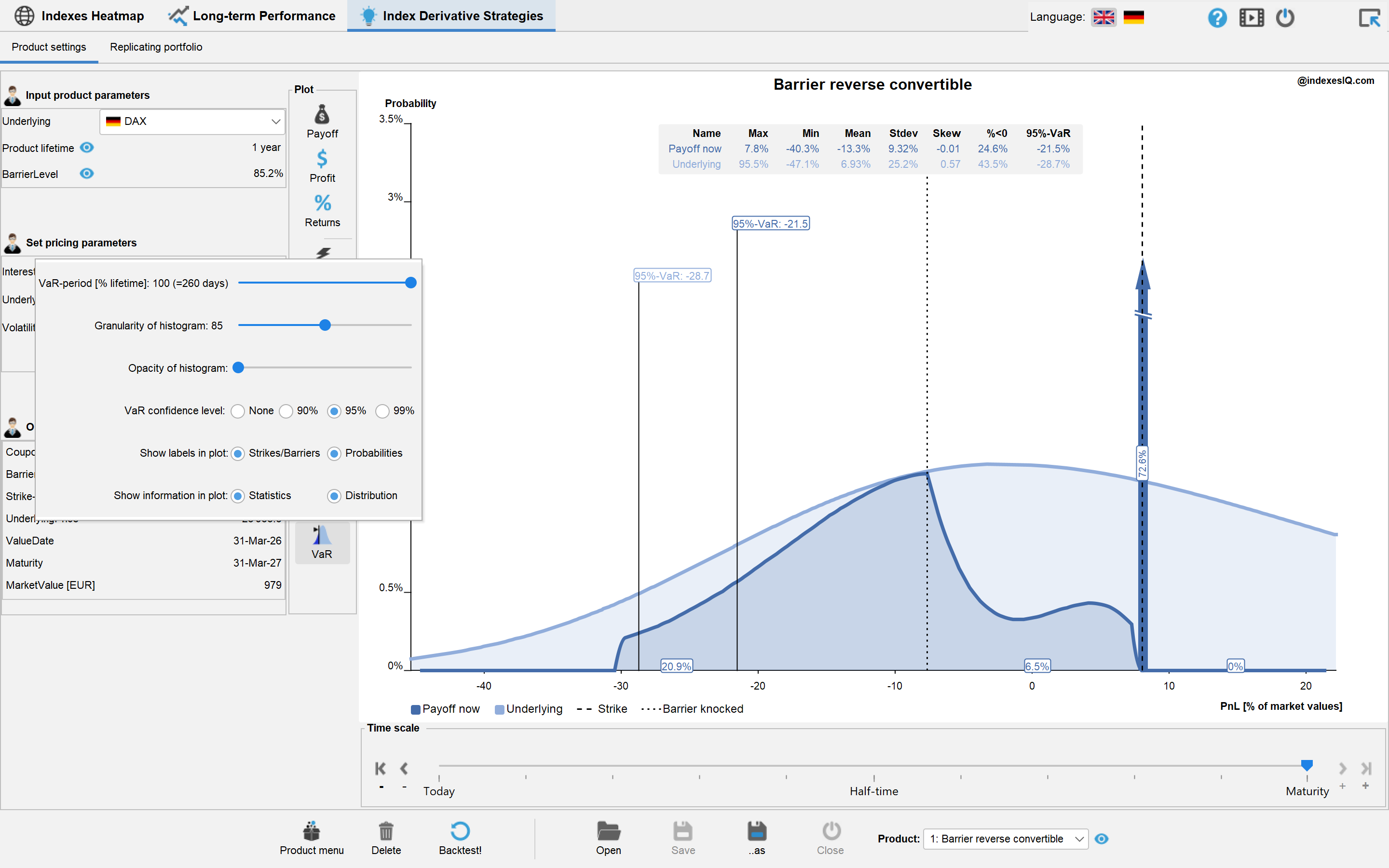
The probability distribution of returns changes during a product's lifetime, which you can simulate using the time-scale function. This is explained conceptually in Chapter 2 of the Derivative Academy.

Product Deep-Dive

After selecting a structured product, the main window shows two panes:

• Products settings pane: Change the basic product parameters such as time to maturity, strikes etc., as well as market price parameters.
• Structuring pane: Define the replicating portfolio and related replication rules. This is for advanced users familiar with structured product replication — as covered in Chapter 3 of the Derivative Academy.

Product Settings Pane

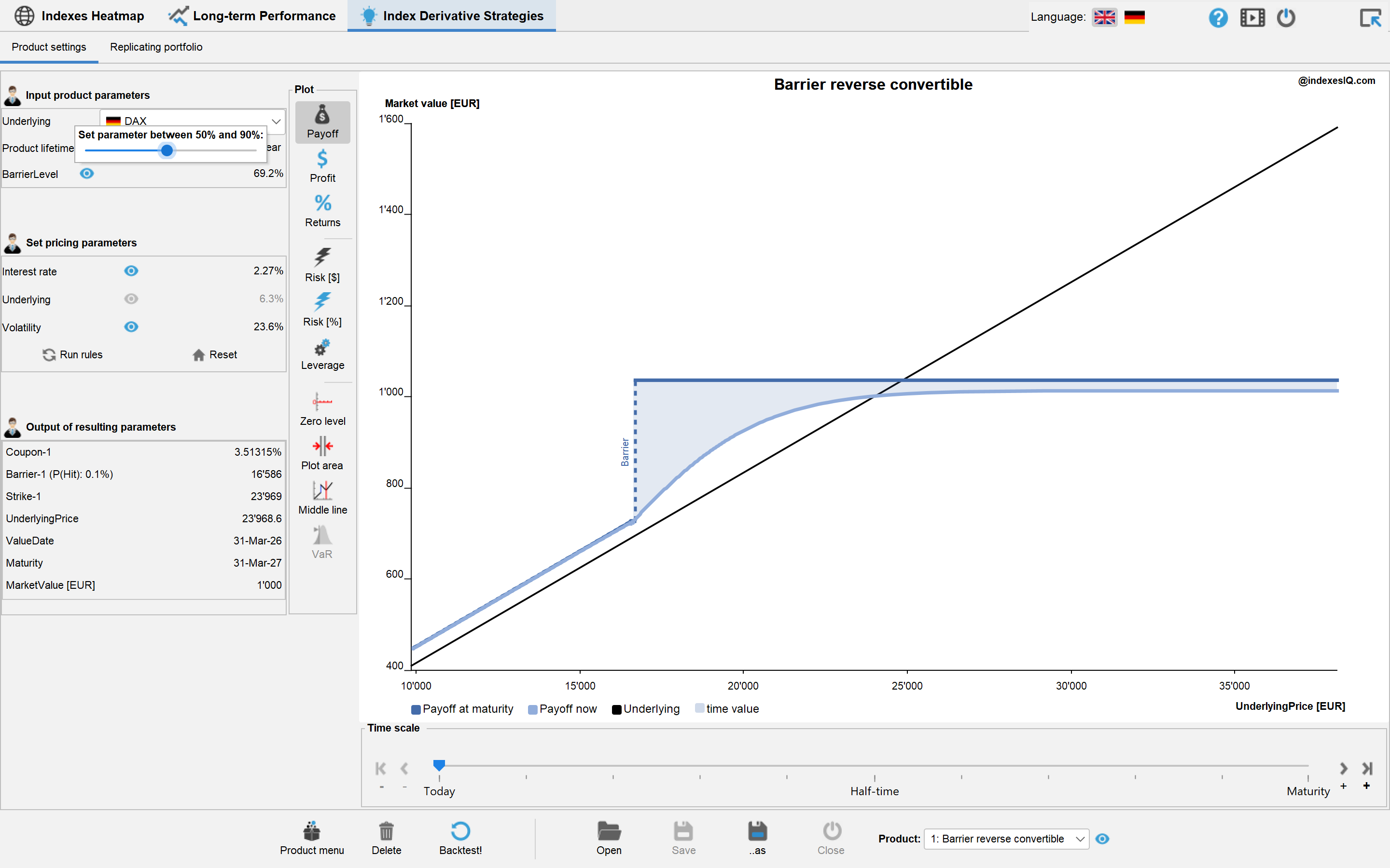
On the left-hand side there are three areas:

Input product parameters — change product parameters such as the lifetime of the product in years or the strike and barrier levels in % of the underlying price at issuance. Click the symbol next to a parameter name to open a pop-up scroll bar. The underlying asset can also be selected here — choices include the S&P 500, EuroStoxx 50, DAX and others. This choice affects both the default market pricing parameters and the historical backtest.

Set pricing parameters — change market price parameters such as the level of interest rates or the volatility of the underlying asset. Standard settings are set to the long-term averages of the chosen underlying asset.

Output of resulting parameters — shows calculated product parameters (actual strike levels, maturity date, product price, Value-at-Risk). Any change in product or market parameters automatically triggers a recalculation including the product plot.

Structuring Pane

The structuring pane is for expert users who want to create new structured products using advanced modelling techniques. Each product is modelled by a replicating portfolio of basic investment instruments and structuring rules — see the Derivative Academy chapter on ingredients for the conceptual background on replicating portfolios.

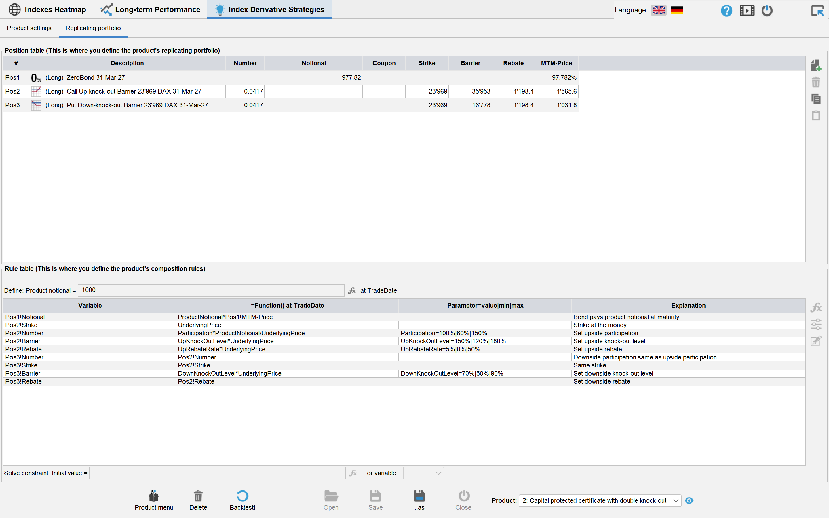
The structuring pane contains two tables:

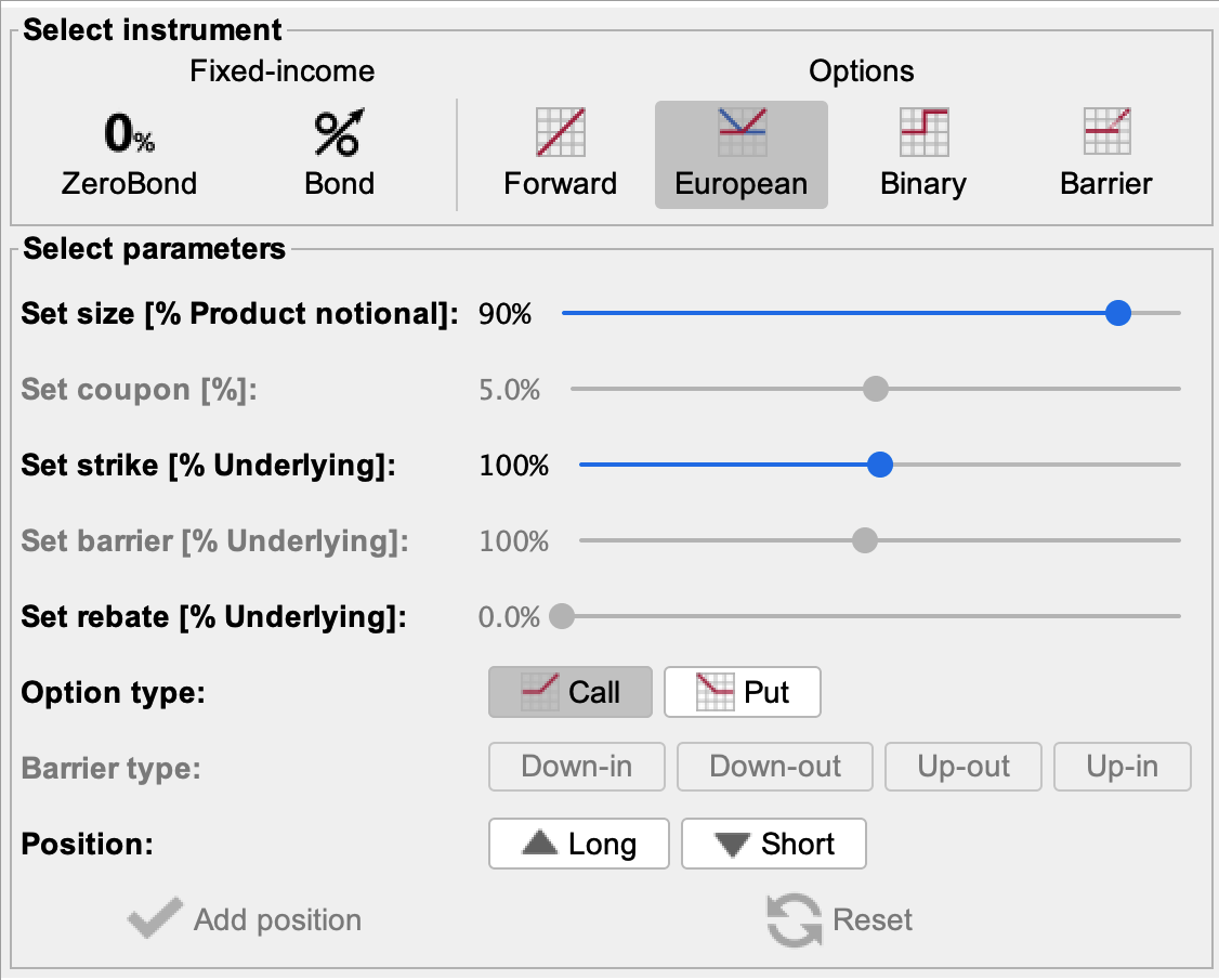
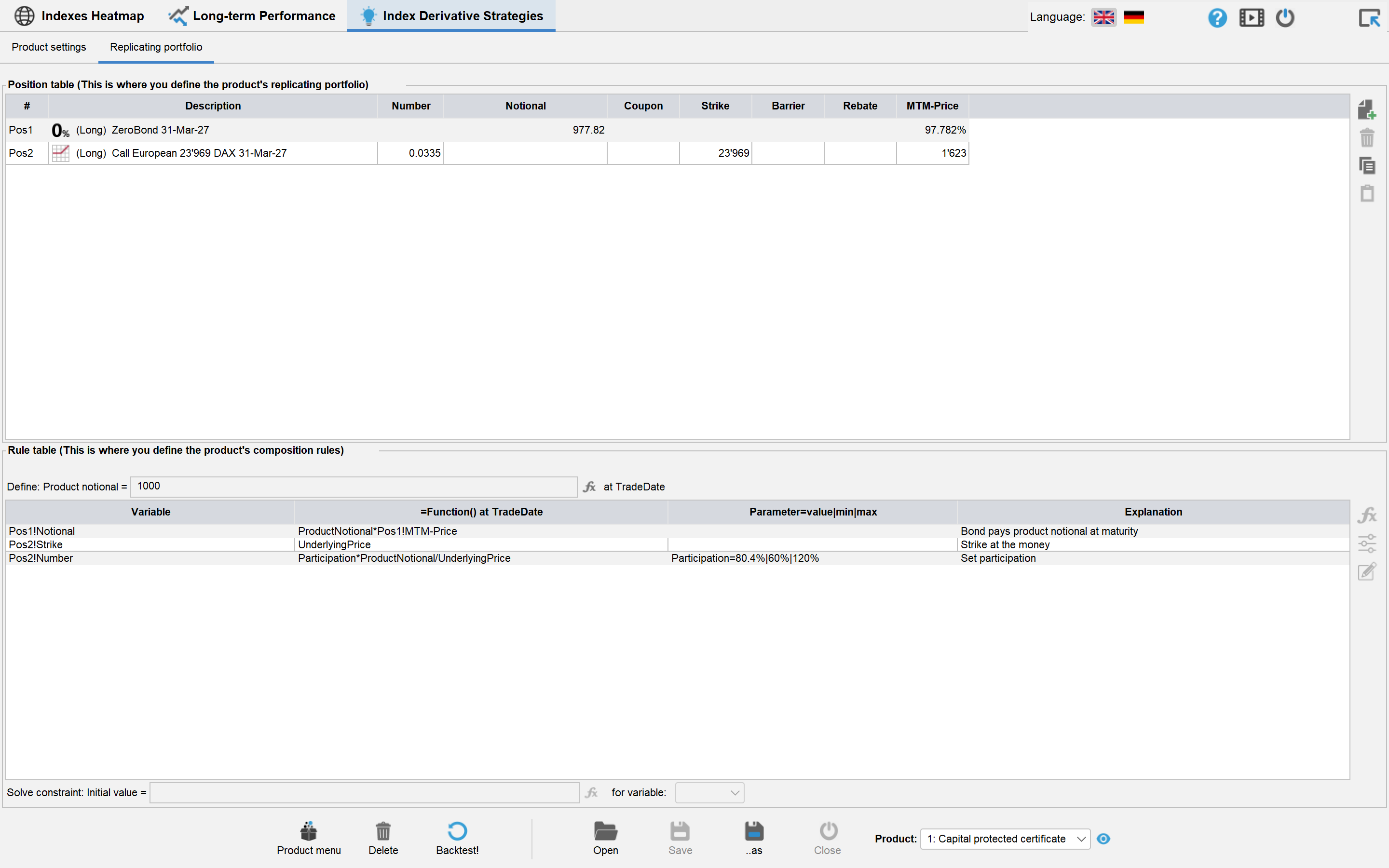
1. The position table (upper) shows the positions that make up the structured product (the replicating portfolio), numbered Pos1, Pos2, etc.

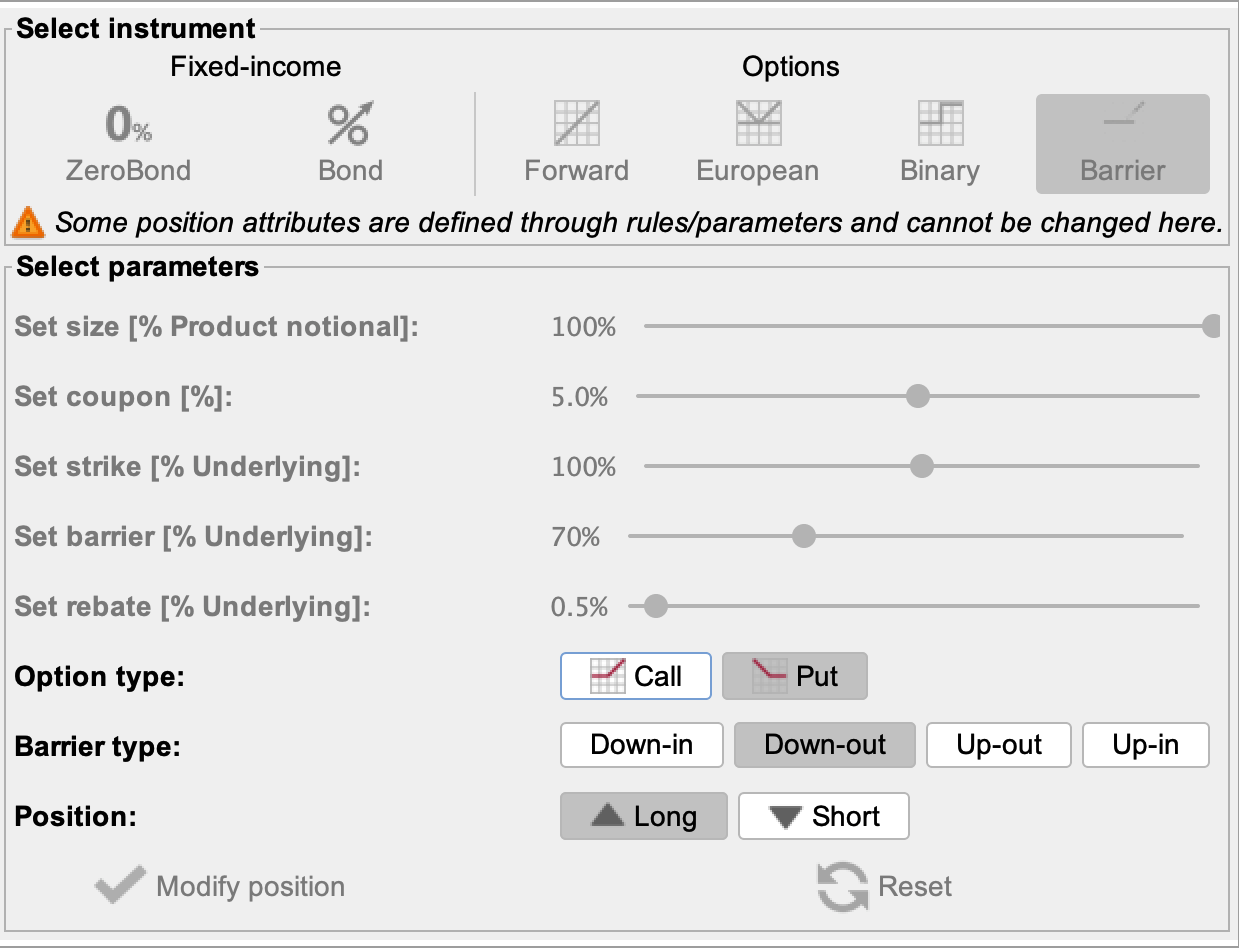
2. The rule table (lower) contains rules defining the basic position parameters. It has four columns:

1. The variable defined by the rule — e.g. Pos1!Strike is the strike price of the instrument called Pos1.
2. The formula used to calculate the variable at ValueDate.
3. Product parameters (see below).
4. A comment explaining the calculation rule.

Rules are managed by the following functions:

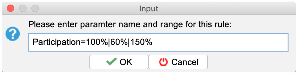
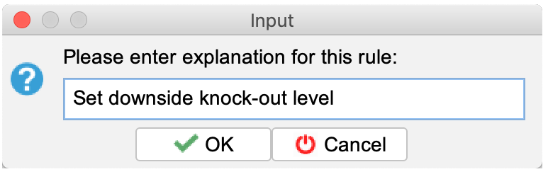
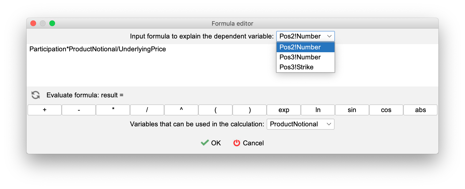
Structuring Example — Capital Protected Note

As a concrete example, consider a capital protected note using a zero-bond (Pos1) and a call option (Pos2). The challenge is to set the contract size of each instrument relative to the product notional and to set the call's strike. For the theoretical background on this construction, see Chapter 4 of the Derivative Academy.

We define a flexible Participation parameter: Participation = 80% | 60% | 120% (initial value 80%, range 60%–120%).

The rules to enter are:

For educational purposes only. Not investment advice.